Spreading Rates and Stokes Number in Dense High Speed Jet Flow: Part 1

This is going to the beginning of me posting about Stokes number and its affect on spreading rates in dense high speed slurry jet flow. This topic is quite extensive and so I’ll break this up into a series of posts so that it is more manageable. This is a significant portion of my dissertation and so writing about this helps me on my side and hopefully it will help other people as well.

I experienced an interesting phenomenon when running simulations at greater than 30% solids by mass (defined by mp/(mp+mf) in my fully coupled three-phase VOF-DEM simulations where spreading rates of the jets significantly increased. Along with this, fluid and particle kinetic energy increased. Now this wasn’t just a slight or linear increase. I would have relatively “straight” flow with little difference between 0-30% solids but then when raised to 40% solids there was a sharp increase in spreading rates and overall system turbulence.

In these simulations I am running 150 micron particles at a bulk fluid (water at room temperature) velocity of 20 m/s through a 6.35mm 5 degree nozzle. We will call this case_set1. What is going on here? Now I’m sure that this has to do with the momentum coupling between the two phases with a significant amount of turbulence generated with increased mass fraction, that one is the first most obvious engineering conclusion. That being said, I had run some previous nozzle-nozzle simulations using 700 micron particles through a 19mm nozzle at bulk velocity of 15m/s (we will call this case_set2) and I was experiencing this same behavior of drastic changes in spreading rates at 30% solids instead of 40% solids and so I also know that we have influences including particle size, fluid properties, and nozzle shape. This brings up the affect of Stokes number on spreading rates and how it relates to increasing percentage of solids.

We know that Stokes number is defined by the ratio of particle and fluid (or eddy) response time. It is a good measure on whether the particle will “go its own path” or follow the flow. There are varying ways to calculate the eddy response time, as pointed out by Lau and Nathan 2016 and Monchaux et al. 2012 [1][2], and I will create a post about this in the future. For now we will categorize our two different flows by the classical nozzle exit Stokes number given by

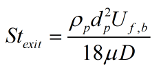
where is the particle density, is the mean particle diameter, is the fluid bulk velocity, is the fluid viscosity, and is the nozzle diameter. Now calculating the exit Stokes number for case_set1 we obtain 11 and for case_set2 we obtain 40.This is starting to make more sense. As expected, as we lower the Stokes number we will get a tendency for the particles to follow the flow more and therefore for case_set1 we will be able to increase mass fraction more than case_set2 until we see the higher spreading rates and turbulence. That being said, this doesn’t explain why we experience the change in spreading rates in the first place but only explains, albeit slightly, why we experience a drastic increase in spreading rates for case_set1 with a higher percentage of solids then for case_set2.

Now, this is only the start to this series of posts. I will be diving into Stokes number further with different ways of calculating the Stokes number along with experiments and simulations. We will also discuss the tendency for particle to cluster in highly turbulent regions. The ultimate question is why the sudden increase highly turbulent regions? Where does that come from? Turbophoretic effect? More rabbit holes to come that hopefully will come to some fruition.

References

[1]Lau, T. C. W., and Nathan, G. J., 2016, “The Effect of Stokes Number on Particle Velocity and Concentration Distributions in a Well-Characterised, Turbulent, Co-Flowing Two-Phase Jet,” J. Fluid Mech., 809, pp. 72–110.

[2]Balachandar, S., and Eaton, J. K., 2010, “Turbulent Dispersed Multiphase Flow,” Annu. Rev. Fluid Mech., 42(1), pp. 111–133.