Particle statistics are extremely important for optimization of any industrial scale unit. Particle collision forces and stresses are difficult to quantify in traditional experiential techniques but is very valuable information because it allows Engineering prediction to be realized. For example, we may want a particular type of collision in flow problem. This can include favor over tangential to normal forces. It may not always be the desire to fully break a particle but instead “scrape” off material from composite particles made of soft and hard materials. Collision frequency is also a very valuable piece of information that can easily be realized from CFD-DEM simulations. Therefore making a Python code that does all these calculations is critical.
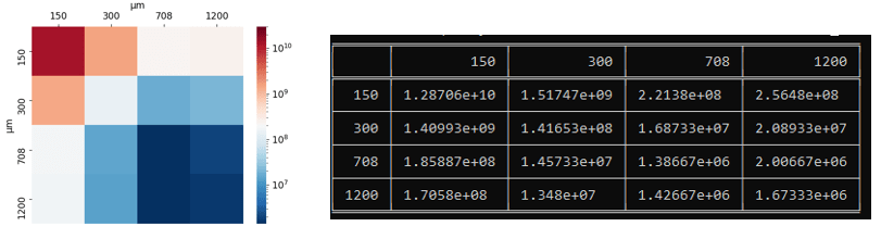
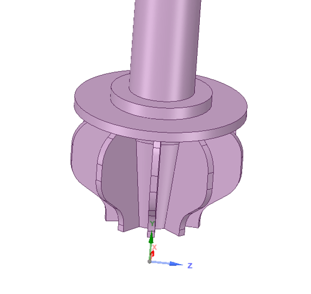
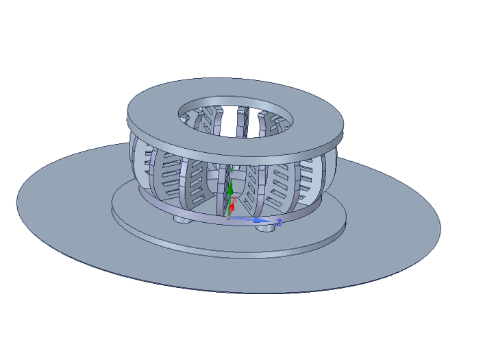
While making a code for outputs of particle statistics is relatively straight forward for simulations with a single particle size, what if we want a particle size distribution (PSD)? This is where filtering comes to view. We need to compartmentalize collisions between particle size fractions while also allowing something that us humans can interpret to further help optimization of the industrial unit. For example, shown in Figure1 is particle collision frequency of a simulation that I have previously performed for the company funding my research (DISA©). We then compare such information between simulations to determine which design we would like. For example, do we want a larger collision frequency of “like” sized particles or do we want more larger particles hitting the smaller ones?
We will want to know collision frequencies and particle collision statistics for force/stresses between all particle size fractions. I therefore created a code that does this in Python. I used Numba for speed and it also has the ability for filtering both by location and by value.
Starting at the simulation level the pairwise velocities, forces, and stresses are computed in the solver of LIGGGHTS© by the adding the following line to the simulation run script
compute frc all pair/gran/local pos vel id force_normal force_tangential contactArea
It should be noted that I have modified the LIGGGHTS© core code to output each particle radius during collision instead of the particle ID. I don’t need ID for my simulations and therefore this makes the most sense. This was easily done by modifying compute_pair_gran_local.cpp starting at line 412 to
    if(idflag)
    {
        radi = atom->radius[i];
        radj = atom->radius[j];
        array[ipair][n++] = radi;
        array[ipair][n++] = radj;
        array[ipair][n++] = 0;
    }
Now we output the particle radius during each collision, and this is used in our Python code.
The Python code starts by inputting all files into memory using the Glob Python package, setting as numpy arrays for contents of each filename, and finally concatenates all the files into a single large numpy array. Some initial calculations and arranging of the array are performed to make it more manageable. This is performed by a function I wrote.
file_list=glob.glob('dump_frc_*')
alldata=read_and_calc(numFiles,file_list)
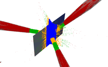
If wanted, this can then by filtered by location. For example, I am filtering out all the collisions occurring at center ,jetstream , nozzle exit, and inner nozzle areas in the follow code snippet.
  centerData = custom_filter(alldata,cn_rxz,0,0.0254)
  jetstreamData = custom_filter(alldata,cn_rxz,0.0254,0.0508)
  nozExitData = custom_filter(alldata,cn_rxz,0.0508,0.0889)
  innerNoz = custom_filter(alldata,cn_rxz,0.0889,0.4445)

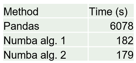
I talked about the custom_filter function in a previous post. This is the most computationally demanding portion of the code because I’m essentially going through each row one by one and filtering, for this case, all particle collision locations with a radius (about the origin) less than a specified value. I tried this before in Pandas and it was ridiculously expensive but now using Numba Python package it is very reasonable by approaching C++ or Fortran speeds.
@nb.jit(nopython=True)
def custom_filter(arr, columnNumber,min,max):

    n, m = arr.shape
    result = np.empty((n, m), dtype=arr.dtype)
    k = 0
    for i in range(n):
        if arr[i, columnNumber] >= min:
          if arr[i, columnNumber] < max:
            result[k, :] = arr[i, :]
            k += 1

    return result[:k, :].copy()
I then collect all collisions in three-dimension Numpy Array with the first two elements of the array being the pairwise collision radius_i and radius_j, and then the third value being whatever value you want specified in that array. For example, it could be the velocity, the force, or the stress.
center_normStress_all = collect_all_collisions(centerData,particle_radii,cn_normStress)
In this code snippet I am taking all collisions in the center region, passing the particle radii of the collisions (the uniques of the collision rows), and specifying that I want the normal stress of these collisions. This gives me the three-dimensional array for the collisions. I then created a function that returns all the statistics of the collisions.
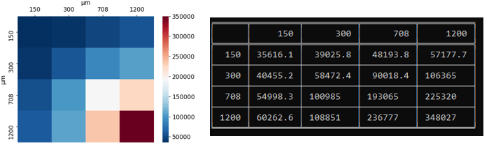
nub_values,min_values,max_values,mean_values,var_values, skew_values,kurtosis_values = describe_all_collisions(center_normStress_all,particle_radii)
This returns 2-dimensional arrays with statistics, and I then print out the table and heatmap by
plot_heatmap(mean_values,uniques,filename = 'center__mean',plot_min = None, plot_max = 350000)

print(tabulate(mean_values, diameters, showindex=diameters, tablefmt="fancy_grid"))
This has proved to be a very valuable tool in my arsenal when analyzing these CFD-DEM simulations. This code will be uploaded to my GitHub if anyone is interested.


 we see that this function is in cfdemCloud.C with the return of

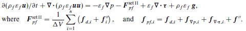
 is is equal to void fraction,
  , for model A (set II) and
  for model Bfull (set II).
 in the code. In CFDEM the calculation of
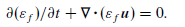
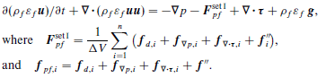
 is the summation of all the particle to fluid interaction forces. To clarify we have for Model A (set II)
 is the particle drag force and
  is the summation of all other forces besides viscous and pressure forces. For example a Saffman lift force would be used here.
 is the viscous force due to intermolecular forces between the particles and fluid, and
  is the pressure gradient force.
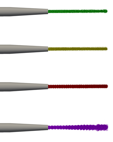
 is the particle density,
  is the mean particle diameter,
  is the fluid bulk velocity,
  is the fluid viscosity, and
  is the nozzle diameter. Now calculating the exit Stokes number for case_set1 we obtain 11 and for case_set2 we obtain 40.This is starting to make more sense. As expected, as we lower the Stokes number we will get a tendency for the particles to follow the flow more and therefore for case_set1 we will be able to increase mass fraction more than case_set2 until we see the higher spreading rates and turbulence. That being said, this doesn’t explain why we experience the change in spreading rates in the first place but only explains, albeit slightly, why we experience a drastic increase in spreading rates for case_set1 with a higher percentage of solids then for case_set2.
 is the volume of partial or full particle (depending on void fraction model) volume. Looking at


 . This method and it’s use is talked about extensively by S. Balachandar and John K. Eaton in their wonderful paper in Annual Review of Fluid Mechanics [1].
